Final - Survival of The Fittest

A Malmo Project for CompSci 175 at UC Irvine

Project Summary

The Survival of the Fittest Project (Our Computer Sciences 175: Project in AI) provides an opportunity for our team to design several agents to survive under a convoluted environment with numerous enemies. From day one, the team has dedicated to an unchanged objective – to find, to design, and to train the best agent to survive in an unpredictable and sophisticated environment, to pursue the goal of longevity.

Essential Knowledge

The project requires us to review, comprehend, and implement what we have learned in CompSci 175, and several other Intelligence System courses – CompSci 171, CompSci 177, and CompSci 178. The project utilized Neural Network and Q-Learning to generate three different agents. Deep Q Network provided the most readily available solution. A neural network delivers an estimation of Q value, and then the agent would determine the best action based on the Q value. Another agent whom the team has been working on is NEAT (Neuroevolution of Augmenting Topologies). NEAT has presented various challenges during the development. It is a powerful method, but the team only has limited knowledge on the subject. The difficulty of working with NEAT prevented use to produce any useful result before the final. Beside Deep Q Network and NEAT, a random agent whose actions are solely determined by unplanned actions without any heuristics. The random one acts as a control group to evaluate the performance of other agents by comparing the performance.

Progress Summary

As described in our Status Report, the team had created an agent with Deep Q Network whom can tackle the task of surviving from one Zombie in a limited cage. Since then, the team has been working on improving the performance of the agent. The MSE – Mean Squared Error – of the Deep Q Network agent shows an ambiguous result, as described in the Status Report. Now, the improvement of performance can be undoubtedly demonstrated by a chart (in-depth demonstration in Evaluation section).

A set of 21 by 21 wall defined the initial playground for the agent and the zombie in the early stage of agent development, while the scope of our agent is only 11 by 11. The limited environment provides a suitable testing ground for our task. Hence, the identical background would repeatedly appear during the training process to a reduce the learning workload for the agents. After the agents could fulfill their task in the predefined environment, the team developed a randomized environment to enlarge the available map space and with more diverse enemy variety.

Approach

Environment Representation / Actions / Reward

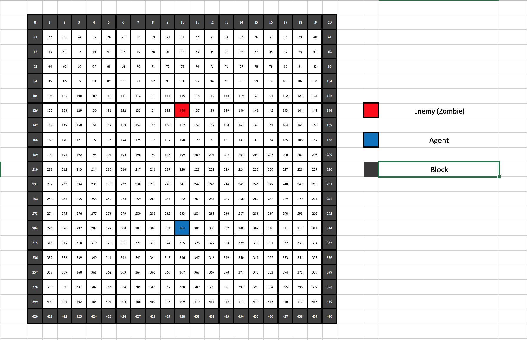
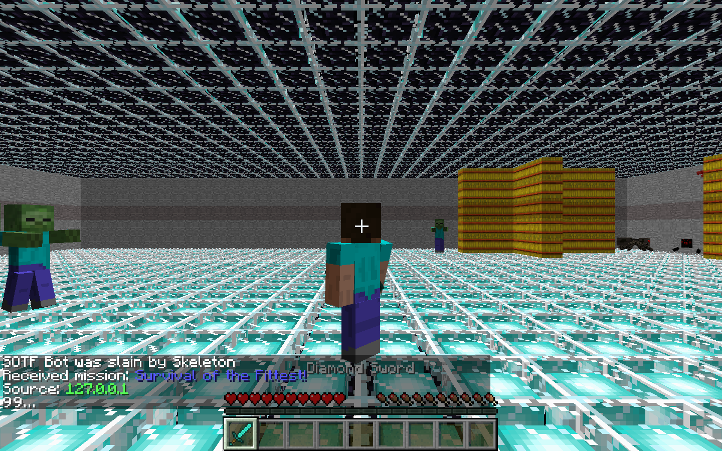
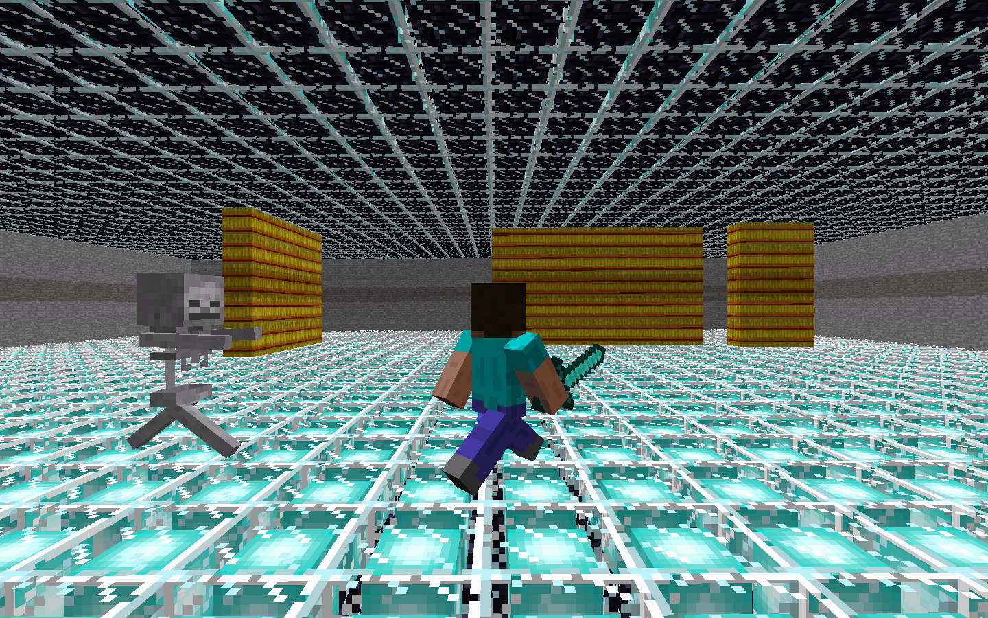
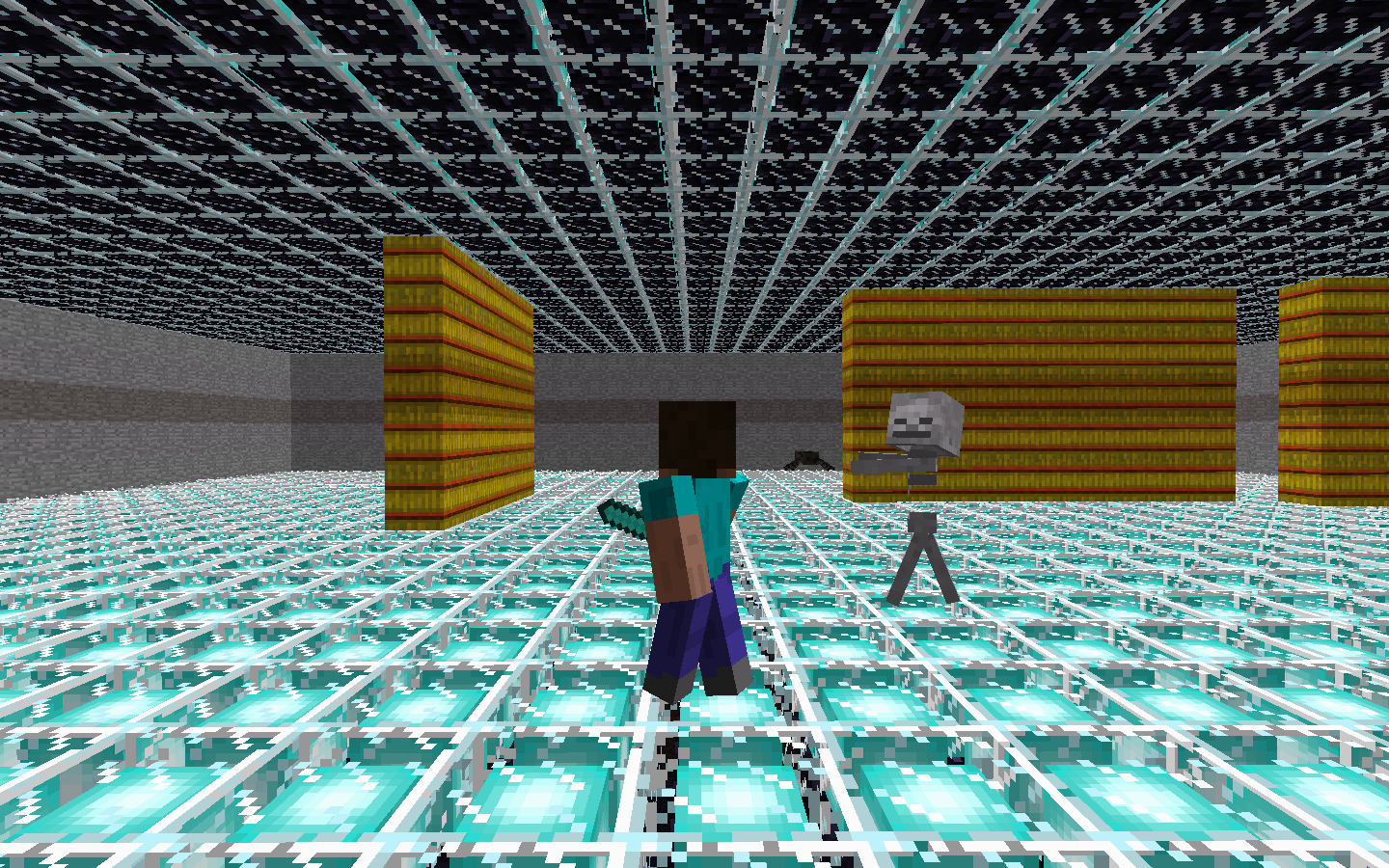
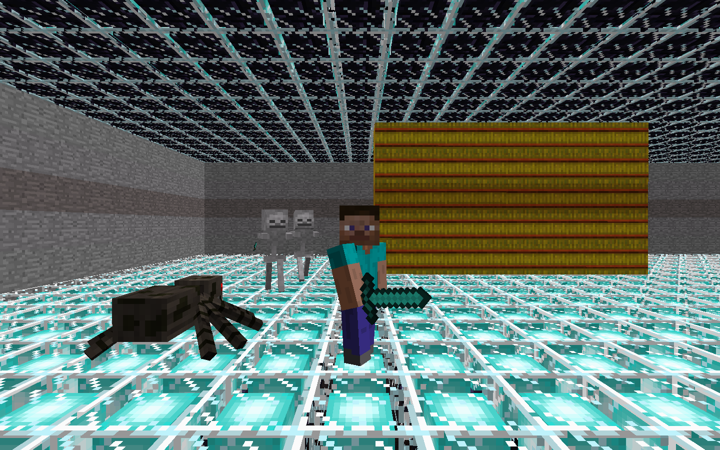
Comparing to the previous version, where our agent tries to survive inside a 21-by-21 cage with one enemy shown as above, our team update the complexity of the environment. We were able to set the environment dynamically based on our needs. For example, in the following images, the environment is configured to be a 41-by-41 cage with stumbling blocks inside the cage. Besides the size of the environment, we also introduce two more types of entities, Spiders, which rarely move but would harm agent if agent steps onto them, and Skeletons, which are mostly identical to Zombies but can move much faster.

Now, our agent automatically converts the 21-by-21 matrix environment to an 11-by-11 matrix to reduce the effective state space. The agent itself remains located at the center of the matrix (matrix[5][5]). Reduction of the state size help accelerates the training process. But if we have a state space that is too small, the training result will likely to be overfitted. (Will show that later in the Evaluation part)

The reward for each state and action only depends on two criteria: agent’s current health and distance between agent and closest enemy. The distance between nearest wall is no longer a depending criterion because we introduce wall into the updated environment and we would like to see how our agent can utilize wall to escape from the enemies. The agent will be rewarded less if an enemy attacks it and lose health (-0.5). The agent will have points deducted (-0.2) if the distance between the agent and the closest enemy is less than 2.0 and will have more points deducted (-0.3) if the agent chooses a move that shortens the distance between agent and most intimate enemy.

Of course, the agent will be rewarded if it can make a move that increases the distance between enemy (+0.3) and some extra rewards if it is able to keep a long distance for a period of time.

Notes: the total reward is within the range of (-1, +1) becasue we use hyperbolic tangent as the activation function.

Algorithm

Algorithm Illustration

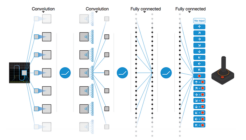
We are using the same algorithm, Deep Q Network algorithm, as we did in previous version to train our agent. Here is a good graphic representation of the training process, excpet we do not need to convolute the game state since we already represent the state with matrix:

The basic idea of Deep Q Network is similar to that of the Q-Learning where we have a reward (Q-Value) associated with a state and each of its corresponding action(s). Then we select the action which possesses the maximum Q-Value among all options.

However, Q Learning is not a feasible approach in our case, since the state is too large and complicated. With a state size of 11 * 11 and three possible entities on each block of map, our program will require gigabytes of space to store a Q-Table (3^121 possible states and 4 actions for each state).

Hence, alternatively, we decided to use Deep Q Network, in which the Q-Function is represented by a Neural Network. It takes the state (matrix)as inputs, and it outputs the Q-Values for each possible action. Finally, the agent can pick the action with the most optimized predicted Q-Value and follow it.

What truly separate Deep Q Network with other reinforcement learning algorithm is its ability to “replay”. The pseudocode of replay function is shown as follow:

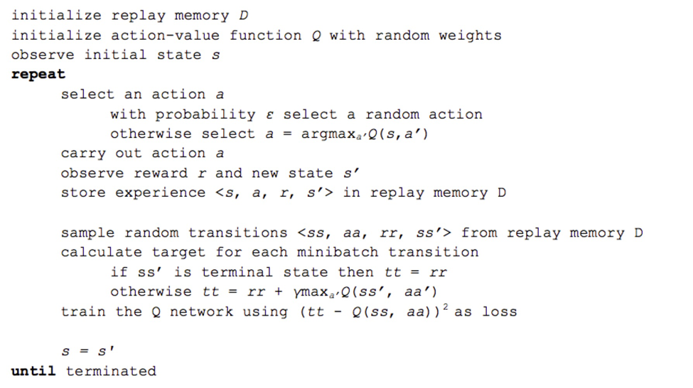
As shown in the pseudocode shown above, the experience <previous_state, previous_action, reward, current_state> is stored each time the agent made a move. To implement this function, we use a list (will probably change to deque in the future) to memory the past experience. Once an episode is ended, a small batch of random experience is retrieved from the list and we use stochastic gradient descent to update the weights of Neutral Network based on these experiences. This method can not only help our agent avoiding local minimum but also improve and stable the agent’s performance since the reward for each state is discrete instead of continuous.

Improvement In Updated Version

In the previous version, for our implementation of Neural Network, we have one input layer with 442 nodes (21 * 21 matrix that represent the current state and 1 value that represent the action), three hidden layers and an output layer with one node. We use hyperbolic tangent as the activation function, so the predicted output will be within the range of (-1, 1).

In the updated version, we changed the size of input layer to a layer with 121 nodes, since the agent converts the visible environment to an 11-by-11 matrix. Then we remove the node that represents action. Instead, we produce an output layer with four values, one for each action (up, down, left, right). A graphic illustration of the new changes would be as follow:

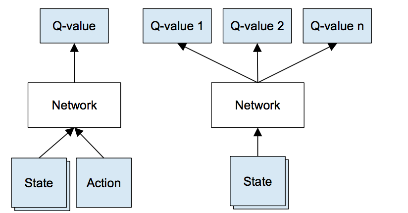
As we stated in the status report, we noticed that, for a given state, the Q-Values predicted for four possible actions are quite similar. The reason for this problem is that, as we use a node in input layer to represent an action, the predictor can hardly distinguish whether it is part of the state or an action and, therefore, produce identical predicted Q-values for all possible actions. After the modification, we can not only guarantee that training improvements can be shared among all possible measure predictions but also make sure that the predictor will provide distinctive Q-Values for each action.

To balance between expolration and exploitation, we introduce Epsilon ( $\epsilon$ -greedy) value, which will decrease as number of episode increases:

   self.epsilon = min(1.0, 1.0/(0.1 * current_episode))

Baseline Agent

Random Action Agent

Agent that choose next action randomly

   def choose_action(self, curr_state, possible_actions):
        if not possible_actions:
            return random.choice(possible_actions)
        else:
            return random.choice([0, 1, 2, 3])

Comparing to our optimal agent, random action agent survive less than 10 seconds.

Mob Fun Agent

Agent that searches for best angles to move based on the surrounding entities (modified based on mob_fun.py provided by Malmo Project)

def getBestAngle(entities, current_yaw, current_health):
    '''Scan through 360 degrees, looking for the best direction in which to take the next step.'''
    us = findUs(entities)
    scores=[]
    # Normalise current yaw:
    while current_yaw < 0:
        current_yaw += 360
    while current_yaw > 360:
        current_yaw -= 360

    # Look for best option
    for i in xrange(agent_search_resolution):
        # Calculate cost of turning:
        ang = 2 * math.pi * (i / float(agent_search_resolution))
        yaw = i * 360.0 / float(agent_search_resolution)
        yawdist = min(abs(yaw-current_yaw), 360-abs(yaw-current_yaw))
        turncost = agent_turn_weight * yawdist
        score = turncost

        # Calculate entity proximity cost for new (x,z):
        x = us.x + agent_stepsize - math.sin(ang)
        z = us.z + agent_stepsize * math.cos(ang)
        for ent in entities:
            dist = (ent.x - x)*(ent.x - x) + (ent.z - z)*(ent.z - z)
            if (dist == 0):
                continue
            weight = 0.0
            if ent.name == MOB_TYPE:
                weight = agent_mob_weight
                dist -= 1   # assume mobs are moving towards us
                if dist <= 0:
                    dist = 0.1
            score += weight / float(dist)

        # Calculate cost of proximity to edges:
        distRight = (2+ARENA_WIDTH/2) - x
        distLeft = (-2-ARENA_WIDTH/2) - x
        distTop = (2+ARENA_BREADTH/2) - z
        distBottom = (-2-ARENA_BREADTH/2) - z
        score += agent_edge_weight / float(distRight * distRight * distRight * distRight)
        score += agent_edge_weight / float(distLeft * distLeft * distLeft * distLeft)
        score += agent_edge_weight / float(distTop * distTop * distTop * distTop)
        score += agent_edge_weight / float(distBottom * distBottom * distBottom * distBottom)
        scores.append(score)

    # Find best score:
    i = scores.index(max(scores))
    # Return as an angle in degrees:
    return i * 360.0 / float(agent_search_resolution)

Comparing to our optimal agent, mob fun agent takes ~0.3 seconds more to produce each action. Also, the surviving time for this agent does not improve as the episode increases.

Evaluation

The evaluation of the agents’ performance bases on two criteria - the average survival time and the Mean Square Error between the actual Q-Value and the predicted Q-Value.

Quantitative Evaluation

MSE for Previous Implementation

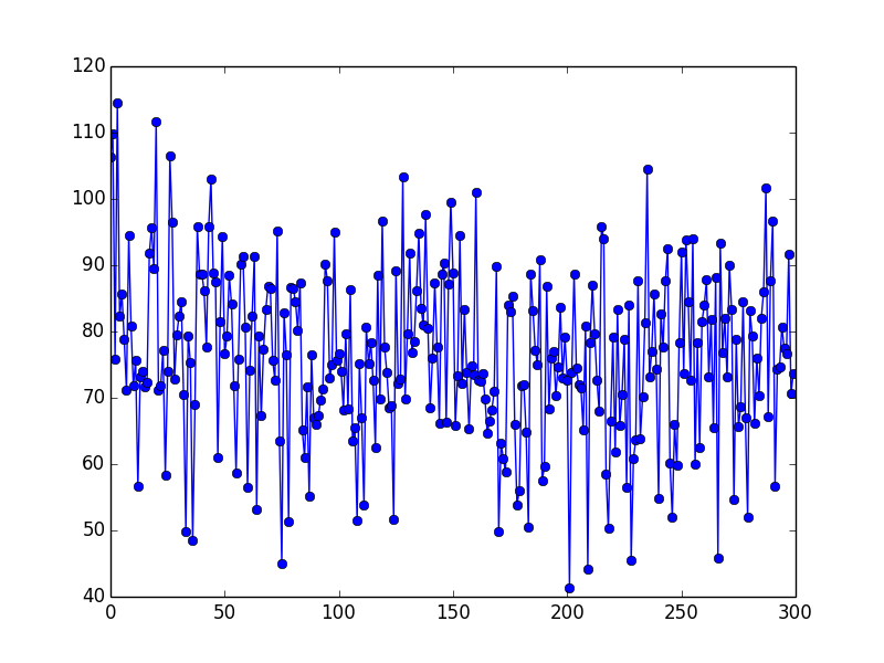
The graph below is the MSE during the training process of our previous implementation. Our agent tried to survive in an environment with size as 11-by-11, no wall and only one Zombie.

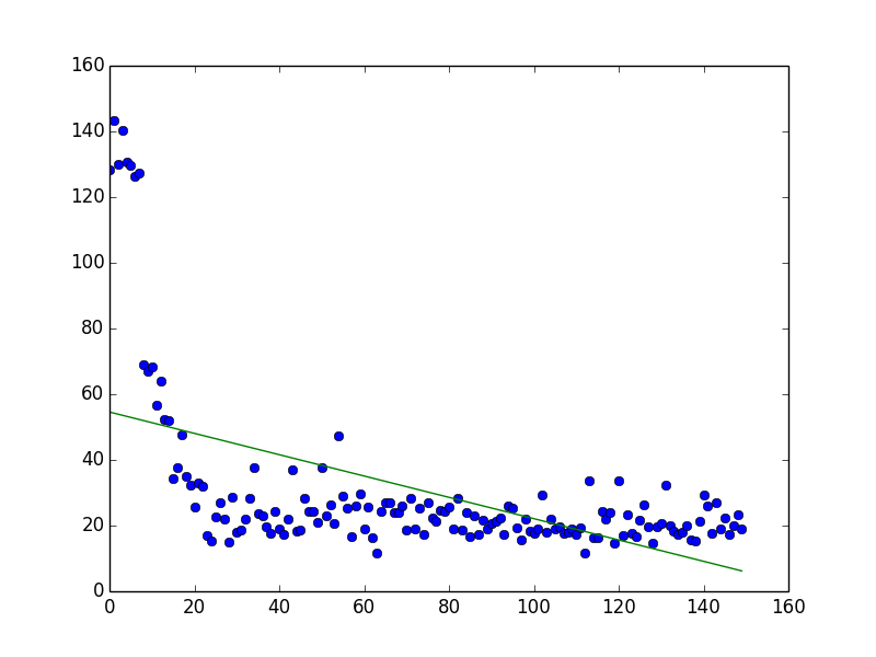
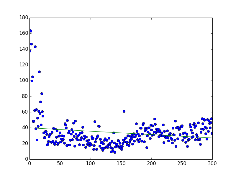
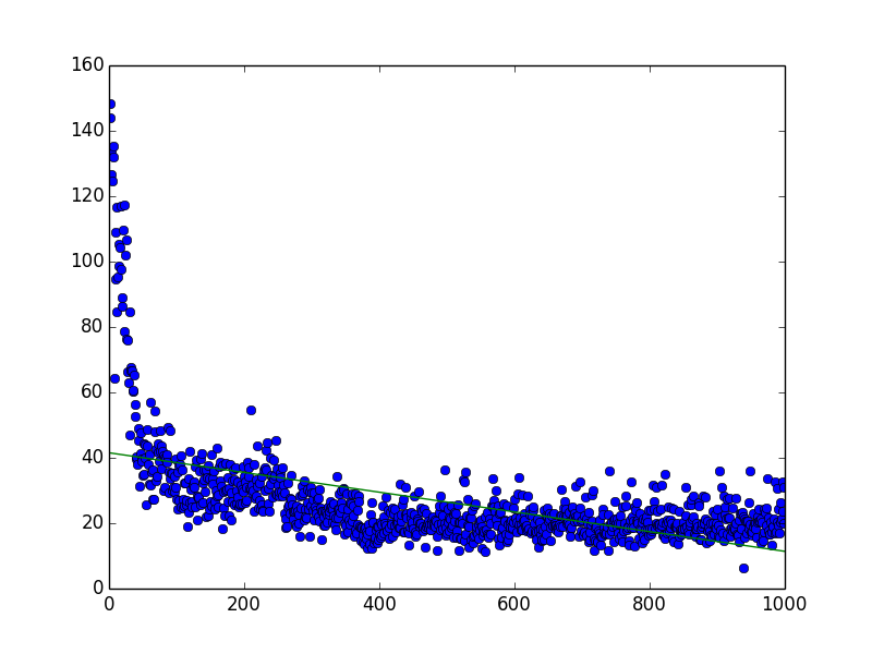
MSE for the Updated Version

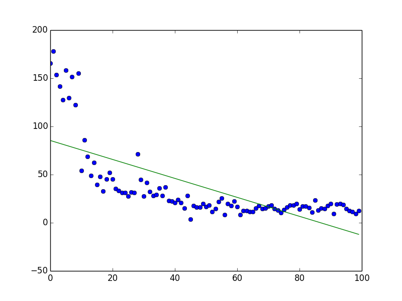
(Complexity: 0, Environment Size: 11 * 11, Number of Enemies: 2, Number of Episodes: 150)

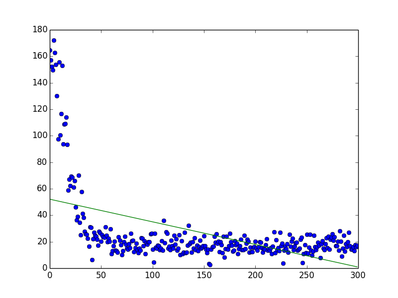
(Complexity: 0, Environment Size: 11 * 11, Number of Enemies: 2, Number of Episodes: 300)

(Complexity: 0, Environment Size: 11 * 11, Number of Enemies: 2, Number of Episodes: 1000)

(Complexity: 5, Environment Size: 21 * 21, Number of Enemies: 5, Number of Episodes: 100)

(Complexity: 5, Environment Size: 21 * 21, Number of Enemies: 5, Number of Episodes: 300)

Notes: To train our agent to survive in a variety of environment, the types of enemies are randomly generated for each episode.

Qualitative Evaluation

Our way to qualitatively evaluate the agent is observing the average survival time for differents types of agent.

Comparing to that of the random action agent, the average survival time of optimal agent is relatively longer. Random action agent usually dies within 10 seconds, while the optimal agent survives up to 100 seconds.
Comparing to that of the random action agent, the average survival time of optimal agent gradually increases as the number of episode increases, which means our agent is learning from past event.
Comparing to the mob fun agent, our agent takes less time to figure the next action given the current states. We conclude this because we can observe clear lag between each action when using mob fun agent.

Reference

Neural Network

Survival of The Fittest CS 175: Project in AI (in Minecraft)